Nešto na našem
Check here different combinations of periods for which to calculate average sea ice extent
Load files
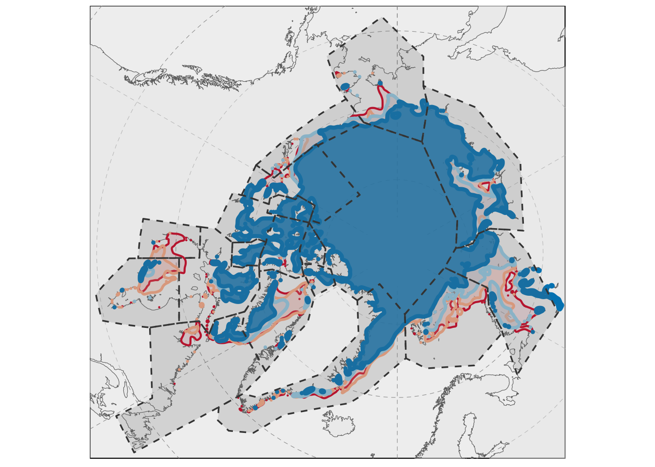
Plot summer extent
polar_bear_spatial_raw %>%
  ggplot() +
  # geom_sf(data = continents_polar, fill = NA, alpha = 0.1) +
  geom_sf(data = continents_polar2, fill = "grey90", alpha = 0.5, lwd = 0.2) +
  geom_sf(data = average_80, color = "#ca0020", lwd = 0.75, fill = "#ca0020", alpha = 0.1) +
  geom_sf(data = average_90, color = "#f4a582", lwd = 1, fill = "#f4a582", alpha = 0.2) +
  geom_sf(data = average_00, color = "#92c5de", lwd = 1.25, fill = "#92c5de", alpha = 0.3) +
  geom_sf(data = average_10, color = "#0571b0", lwd = 1.5, fill = "#0571b0", alpha = 0.8) +
  geom_sf(data = polar_bear_spatial_raw, fill = "grey40", alpha = 0.2, lwd = 0.6, linetype = 2, color = "grey20") +
  # geom_sf_label(aes(label = Subpopulation_abbr, size = 2), nudge_x = -2) +
  # coord_sf(xlim = c(-2600000, 2600000), ylim = c(-3500000, 2500000)) + # Sea routes projection
  coord_sf(xlim = c(-4300000, 2200000), ylim = c(-2800000, 3400000)) +
  theme_map() +
  theme(
    panel.grid.major = element_line(color = "grey50", linetype = 2, size = 0.5),
            rect = element_rect(fill = "grey50"),
    panel.background = element_rect(fill = "grey93"),
    # plot.background = element_rect(fill = "transparent", color = NA),
    # panel.grid.major = element_blank(),
    # panel.grid.minor = element_blank(), legend.background = element_rect(fill = "transparent"), legend.box.background = element_rect(fill = "transparent")
    NULL
  ) +
  NULL